Current state of practice in North America to evaluate the performance of slopes during earthquake loading is to use one of the following approaches:

1.  Limit Equilibrium Approach

This approach uses horizontal and vertical seismic coefficients (k_h and k_v) to estimate seismic loads and performs a traditional limit equilibrium analysis to evaluate factor of safety against sliding. Figure 1 below illustrates the approach. A slope is judged to be safe for a design earthquake if the factor of safety is equal to or greater than 1.10 (NCHRP Report 611, 2008 and Olson and Stark, 2003). By using this approach, you can evaluate the slope stability and the potential for any flow failure, however you cannot get a rough estimate of slope deformation.

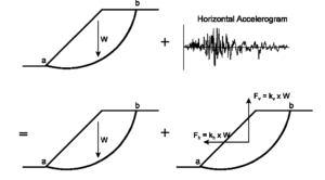
A wide variety of computer programs (e.g. SLOPE/W, SLIDE) are commercially available to perform the required pseudo-static limit equilibrium analysis. The analysis procedure is straight forward, however, determination of a seismic coefficient that can appropriately represent the characteristics of design earthquakes is not easy. It is to be noted that seismic coefficient is not equivalent to the site-adjusted peak ground acceleration (PGA) because acceleration varies in depth of the sliding block and PGA occurs just at its surface. Therefore, the equivalent seismic coefficient should be just a percentage of the site-adjusted PGA. A number of recent publications have provided guidance in the selection of an appropriate seismic coefficient where the coefficient is a function of;

(i) design earthquake characteristics (Magnitude, M, distance from fault, R, peak ground velocity, PGV), and

(ii) lateral displacement of the slope.

The selection of appropriate seismic coefficient relies on both local code requirements and engineering judgement. The procedures outlined below are recommended for determination of seismic coefficient.

1.1. Non-liquefiable site condition

A reliable design approach that you can use is the approach of Bray et al. (1998). It is worth mentioning that SP 117-“Guidelines for evaluating and mitigating seismic hazards in California” recommends the use of this approach to calculate seismic coefficient. The formulation is given as,

k_h=f_{eq} \times MHA_r

where MHA_r is PGA at a rock site condition , and f_{eq} is a factor related to the design earthquake characteristics and threshold lateral displacement of the slope. f_{eq} is given as,

f_{eq}=\frac{NRF}{3.477} \times [ 1.87-log_{10}(\frac{u}{(MHR_r/g)\times NRF \times D_{5-95}})]

where D_{5-95} is median duration calculated per the approach presented by Abrahamson and Silva (1996), NRF is a factor that accounts for the nonlinear response of the soil material above the slide plane,  and u is slope threshold displacement in units of cm. If you are to improve the stability of a slope, u would be the allowable slope deformation prescribed by the project team. If you are to just evaluate deformation of an existing slope, as mentioned above in the beginning of the article this method is NOT suitable. For further elaboration on the equations above please check out Chapter 11 of Recommended Procedures for Implementation of DMG Special Publication 117: Guidelines for Analyzing and Mitigating Landslide Hazards in California (link).

For your convenience, I formulated the above equations in a spreadsheet. You can download it here:  Seismic-Coefficient-Calculator.xlsx

Bray et al (2002) simplified the process of estimating f_{eq} and presented the results of above calculations in a figure (Figure 2 below) for different ranges of earthquake magnitude and distance for two levels of threshold slope displacements, 5 and 15 cm.

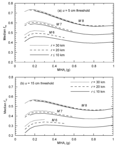
Figure 2. Values of f_{eq} as function of MHA_{r}, earthquake magnitude and fault distance (r) ro threshold displacements of (a) 5cm and (b) 15 cm (SP117, 2008).

1.2. Liquefiable site condition

Although the procedure described above was originally developed for non-liquefiable site condition, it is also used for liquefiable site conditions. There are two main challenges when liquefaction is involved in slope stability analysis;

(i) determination of representative soil parameters to appropriately approximate soil softening and strength loss during  liquefaction;

(ii) determination of representative seismic coefficient. Note that liquefaction generally triggers after the strongest motion pulses of an earthquake hit the liquefiable layer. To this end, some percentage of the seismic coefficient calculated per the procedure described in the previous section should be used for slope stability (0.0 \leq k_{h, liq} < k_{h}) .

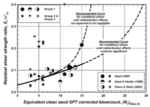
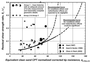
Regarding item (i); in the current state of practice, soil stiffness/strength degradation of liquefied soil is represented by using soil residual strength in the slope stability analysis. The residual strength can be estimated per the SPT- and CPT-based correlations recommended by Idriss and Boulanger (2008). See Figure 3 to determine the residual shear strengths.

Regarding item (ii); using k_{h, liq} = k_{h} in a slope stability analysis would result in too conservative design since liquefaction state and peak ground acceleration do not occur simultaneously. However, it is to be noted that there is high level of conservatism incorporated into prediction of liquefaction triggering, peak ground acceleration (PGA), earthquake magnitude (M), and residual shear strength of liquefied soil. To this end, using   k_{h, liq} = 0.0 in slope stability analysis seems to be appropriate. Most of the geotechnical consulting firms use k_{h, liq} = 0.0 for liquefiable soil condition.

2.  Displacement-Based Approach

This approach includes either the simplified Newmark sliding block concept or advanced continuum modeling method. This article will focus on Newmark sliding block approach only. Advanced continuum modeling method is briefly discussed in here.

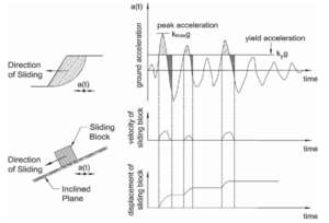
The Newmark sliding block method treats the potential failure mass as a rigid body resting on a failure plane. When the input ground motion induced along the failure plane exceeds a threshold acceleration, deformations accumulate over time resulting in residual slope deformations (see Figure 5). The threshold acceleration is also called yield acceleration (k_{y}) and is defined as the horizontal acceleration that results in a factor of safety of 1.0 in a pseudo-static limit equilibrium analysis.

The method is shown to be a function of earthquake characteristics such as magnitude (M), PGA, PGV, and distance from fault. Accordingly, based on this approach several research groups performed statistical analysis for a wide range of historical earthquake motions and developed equations to calculate slope deformation as a function of k_{y} and site-adjusted earthquake characteristics. Most of these equations have been nicely formulated in the computer program SLAMMER. In case you do not want to use the equations, this program can also perform Newmark sliding block analysis for a suite of ground motion time histories.

One drawback of the original sliding block model is that it treats the failure mass as a rigid body and ignores deformability of the sliding block. Seed and Martin (1966) and Makdisi and Seed (1978) showed that the method does not capture accurately the dynamic response of  the deformable earth/waste sliding mass during earthquake shaking. Bray and Travasaro (2007) proposed a method that takes into account deformability of the sliding block. The method is also available in the computer program SLAMMER.

2.1. Non-liquefiable site condition

As discussed above the analysis is completed in the following three steps:

1. Determine yield acceleration (k_{y}): perform pseudo-static limit equilibrium analyses iteratively by varying k_{h} values. The k_{h} that results in safety factor of 1.0 would be the yield acceleration,
2. Determine characteristics of design earthquakes for the site in question,
3. Use computer programs such as SLAMMER to calculate slope deformations. If the slope is composed of soft material, it is recommended to use the approach of  Bray and Travasaro (2007) since it accounts for failure mass deformability. If the slope is composed of stiff/dense material underlain by a very soft layer, it is recommended to also consider Newmark sliding rigid  block.

2.2. Liquefiable site condition

The analysis includes the steps listed above with two major changes:

• Residual shear strength of liquefiable layers must be used in the limit equilibrium analysis to calculate k_{y};
• Bray and Travasaro (2007) method should NOT be used because the sliding mass behavior is more like a rigid body resting on a liquefied soil. It is recommended to use Newmark sliding rigid  block.

There are some empirical methods available to estimate liquefaction-induced lateral displacements based on standard penetration test (SPT) and cone penetration test (CPT), e.g., Youd et al. (2002) and Zhang et al. (2004). These methods are not discussed here for brevity, and note that the methods are NOT applicable if you intend to find a solution to stabilize a slope by some techniques such as soil-nailing, piles, deep soil mixing buttress, etc.

3.  Concluding Remarks

The displacement-based approach has two advantages over the limit equilibrium approach:

1. Unlike limit equilibrium approach, the displacement-based approach provides rough estimate of a slope deformation.
2.  In displacement-based approach, there is no need to estimate seismic coefficient (k_{h}).

Last but not the least, in my opinion both methods described above are approximate and can be associated with some level of error. The most reliable tool for this purpose is to adopt advanced numerical approaches and simulate full-scale continuum model of the system in question. This way there is no need to; (i) estimate pseudo-static seismic coefficient, (ii) estimate residual strength of liquefied soils, and (iii) make any engineering judgment on the level of deformability of potential sliding masses.

Important Note:

The methods described above were originally developed and formulated for shallow crustal earthquake events, and characteristics of subduction zone earthquakes were NOT incorporated in those approaches. Very recent studies such as the study of Bray et al. (2017) provides recommendations on calculation of lateral displacement of slopes when subjected to subduction zone earthquakes. They have incorporated their approaches including the 2007 version (Bray and Travasarou, 2007) in a spreadsheet which is available online for free. The spreadsheet is also capable of estimating the seismic coefficient (k_{h}).

For ease of access, I have uploaded the spreadsheet here in the following link:  BT07_BMT17_Seismic_Slope_Displacement_v5.xlsx
(by Bray et al. 2017).