Common simplified approaches to calculate seismic active pressure are described below:

1. Semi-empirical Mononobe-Okabe Method

The simplest method to approximate seismic active pressure is to use the approach of Mononobe-Okabe (M-O) which is originally based on Coulomb’s theory of static earth pressures. The method incorporates the following assumptions (Geraili and Sitar, 2013):

• The backfill soil is dry, cohesionless, isotropic, homogenous and elastically undeformable material with a constant internal friction angle;
• The potential failure surface in the backfill is a plane that goes through the heel of the wall;
• The wall is long enough to make the end effect negligible;
• Sufficient rigid body displacement is required to mobilize the active wedge in the soil.

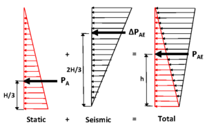
The M-O method was modified by Seed and Whitman (1970) for easier application in the practice. They proposed to separate the M-O seismic active pressure into two components; (i) active static component (P_{A}), and  (ii) seismic increment of active earth pressure (\Delta P_{AE}). P_{A} is calculated using the static Coulomb theory for static and is applied at H/3 from the wall base. Per Seed and Whitman’s (1970) parametric analyses results,  \Delta P_{AE} is given as,

\Delta k_{AE} = \frac{3}{4} k_{h}
\Delta P_{AE} = \frac{1}{2} \gamma H^2 \Delta k_{AE} = \frac{3}{8} \gamma H^2 k_h

where \gamma is backfill soil unit weight, H is the height of retaining structure, and k_h is seismic coefficient. You can appropriately estimate the k_h value by using the procedure described here in section 1.1.

Figure 1 below presents a better illustration of the seismic pressure distributions. Per Seed and Whitman (1970),  \Delta P_{AE} is applied at 2/3H above the base of the wall (i.e., inverted triangular pressure distribution).

The method has several limitations that stem from the four assumptions listed above. The method may not provide realistic estimations of seismic pressures if the retaining structure is flexible and soil material behind the wall is cohesive and/or nonuniform. In addition, the method estimates some levels of earth pressure at the ground surface which is not realistic.

In my opinion due to the complexity of the problem, the seismic active pressure needs to be calculated using advanced numerical methods by analyzing a full-scale continuum model of the retaining structure and the retained soil domain. However, this approach may not be accepted by some project design teams due to shortage of time or limited access to advanced computational tools. In such cases, some geotechnical consulting firms use an alternative approach which is, in my opinion, more reliable than the M-O method. The approach is elaborated below.

2. Limit Equilibrium Method

This approach requires performing iterative 2D limit equilibrium slope stability analysis using any of the available commercial softwares such as SLIDE, SLOPE/W, etc. To approximate the seismic active pressure you need to follow the procedure below:

1. Estimate seismic coefficient k_h using the procedure described here in section 1.1;
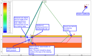
2. Develop a model of retaining structure and soil layers (see Figure 2 below) using computer program SLIDE, SLOPE/W, etc;
3. Remove the retaining structure from the model and remove some soil volume in front face of retaining structure with the same height of the structure as shown in Figure 2.  The width of the removed area can be any random value because the goal is just to eliminate shear and normal stresses at the interface of the retaining structure and the retained soil;
4. Define a triangular soil pressure applied horizontally in the opposite direction of the seismic coefficient. The pressure should be applied over the entire height of the retaining structure (see Figure 2). Note that the retaining system should be removed from the model. The analysis is going to be conducted iteratively by varying the soil pressure, so for now, use a random pressure, e.g., 2000 psf;
5. Define failure plane search box behind the retaining structure and a single search point at the toe. See Figure 2 for better illustration;
6. Perform limit equilibrium analysis iteratively by varying soil pressure (defined in step 4) until factor of safety against failure becomes 1.10. The pressure corresponding to FoS=1.10 is considered as total seismic active pressure (P_{AE}) which is applied at H/3 from the base.