Introduction
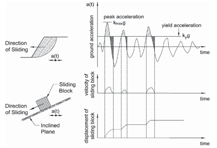
Practitioners often perform Newmark Sliding Block analyses to predict permanent lateral displacements of slopes under earthquake loading. In this method, sliding of a rigid block of soil mass is computed by double integration of acceleration over the length of time during which the yield acceleration (i.e., friction coefficient) is exceeded. For better illustration purposes, schematics of this procedure is shown in Figure 1 below.
This model may be interchangeably referred to as “conventional Newmark model” and “rigid block model” in the current literature. Although the model is simple and uses a series of site-specific ground motion time histories to determine potential slope movements, it neglects the dynamic response, i.e., deformability, of the sliding mass above a potential failure surface during shaking.
To account for deformability and flexibility of the sliding block, Kramer and Smith (1997) proposed a “modified Newmark model” in which the soil block is replaced by 2 or more smaller blocks of soils connected by springs and dashpots. The shear resistance at the base of the model is NOT allowed to exceed the friction ratio times the total weight of the soil blocks. The springs, dashpot, and the soil blocks are meant to approximate the dynamic characteristics of the sliding block.
Modified Newmark Model
Figure 2 illustrates some details of the modified Newmark model. As mentioned earlier, the sliding soil block is represented by 2 or more smaller blocks of soils connected by springs and dashpots.
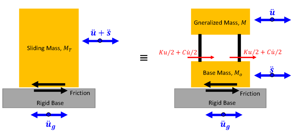
According to Kramer and Smith (1997), equilibrium for the upper mass (M) is expressed as:
M\ddot u+K u+C\dot u=-M(\ddot u_g+\ddot s) …………….. (Eqn. 1)
And the equilibrium for the lower mass (M_o) is given by:
K u+C\dot u-k_y(M+M_o)g=M_o(\ddot u_g+\ddot s) ……. (Eqn. 2)
where K and C represent stiffness and damping of the deformable sliding mass, respectively; \ddot s is the sliding acceleration, k_y is the yield acceleration (the friction coefficient along the sliding interface), M represents the portion of the total mass (M_T) that responds dynamically, and M_o is M_T-M.
M can be obtained by calculating the generalized mass which is expressed as:
M=\int_{0}^{H'} m(z)\phi_n^2 \,dz …………………………………. (Eqn. 3)
where m(z) is the distribution of mass along the soil height z , H' is the height of the sliding mass and \phi_n is the mode shape function for the n^{th} mode. For a linear elastic half-space \phi_n can be given by:
\phi_n=sin(\frac{(2n-1) \pi z}{2H'}) ………………………………… (Eqn. 4)
Combining Eqn. 4 with Eqn. 3:
M=M_T/2
The above was formulated in a MATLAB code to solve equilibrium equations of a stick-slip sliding single-degree of freedom (SDOF) under an earthquake ground motion.
The MATLAB “.m” file can be downloaded from this link:
Download link:
MATLAB-Deformable Sliding Block Model
In this MATLAB file:
1. The fundamental vibration period (T_s) of the sliding mass was estimated by:
T_s=4H'/V_s ………………………………… Eqn. (5)
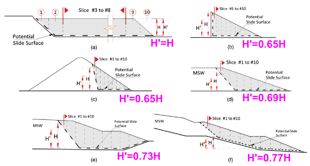
where V_s is the average shear wave velocity of the soil profile within the sliding block, and H' is the effective height of the sliding mass per Bray and Macedo (2019). Their recommended effective heights for different configuration of the slope is presented in Figure 3. For more details please visit Bray and Macedo (2019).
2. Both linear and equivalent linear elastic approaches can be used. For linear elastic analysis, G/G_{max} can be defined as [1.0 1.0] for shear strains of [0 10%].
3. Similar to the Conventional Newmark model, sliding is accumulated in one direction (downslope) only and sliding in the opposite direction (upslope) is set to zero.
4. Lines 67 to 83 of the MATLAB file read input ground motions (accelerations in ‘g’ unit). These lines may need to be modified based on the format of your input files.
5. Conventional Newmark model (rigid block model) can be also simulated by using a sufficiently large shear wave velocity for the sliding block (e.g., 1e10 ft/sec).
Validation
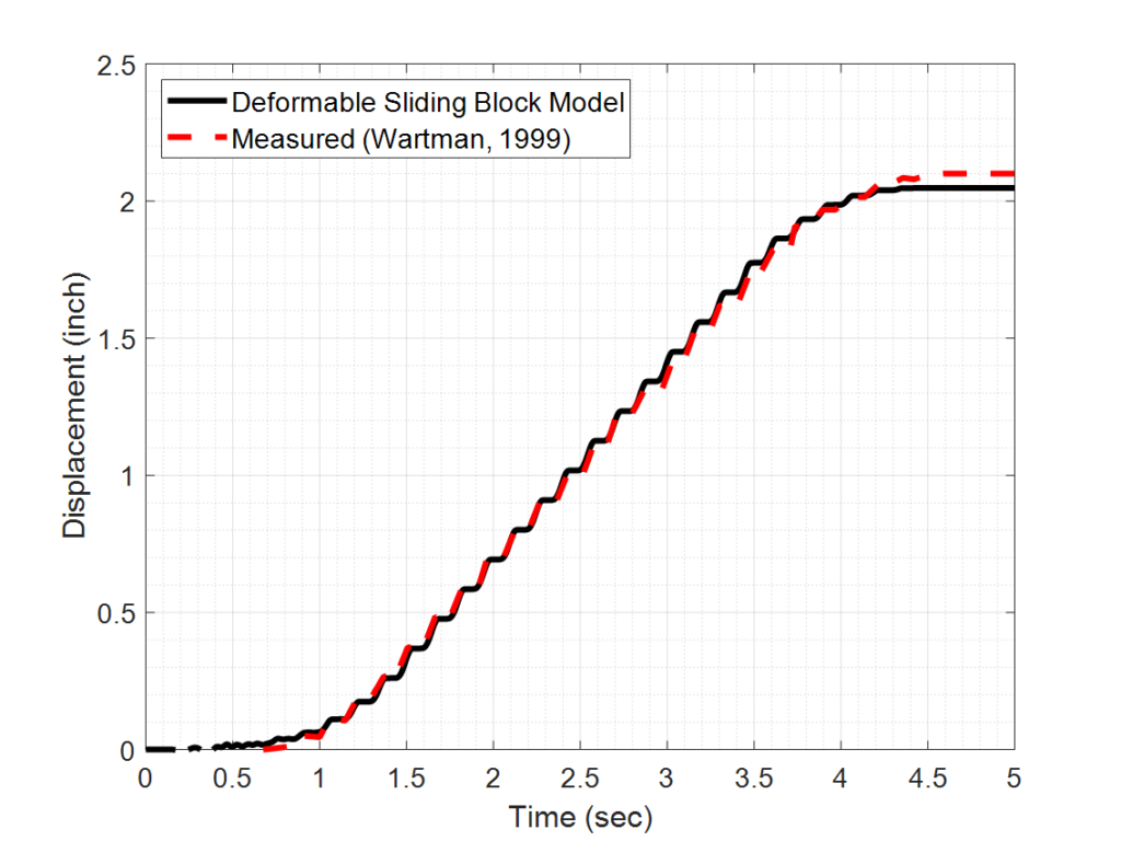
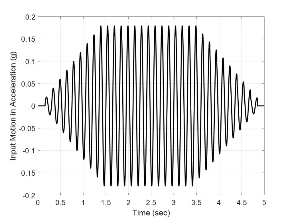
The MATLAB code was validated against results from shaking table experiments performed by Wartman et. al (2005) on a deformable soil column consisted of kaolinite/bentonite clay. For brevity, the details of the shaking table test are not presented here. Details of the test can be found in Wartman et. al (2005). Figure 4 shows the comparison of the computed and measured soil column displacement under a 6.7-Hz sinusoidal motion with a maximum horizontal acceleration of 0.18g (see Figure 5). The results indicate that the model is capable of capturing the measured displacements.
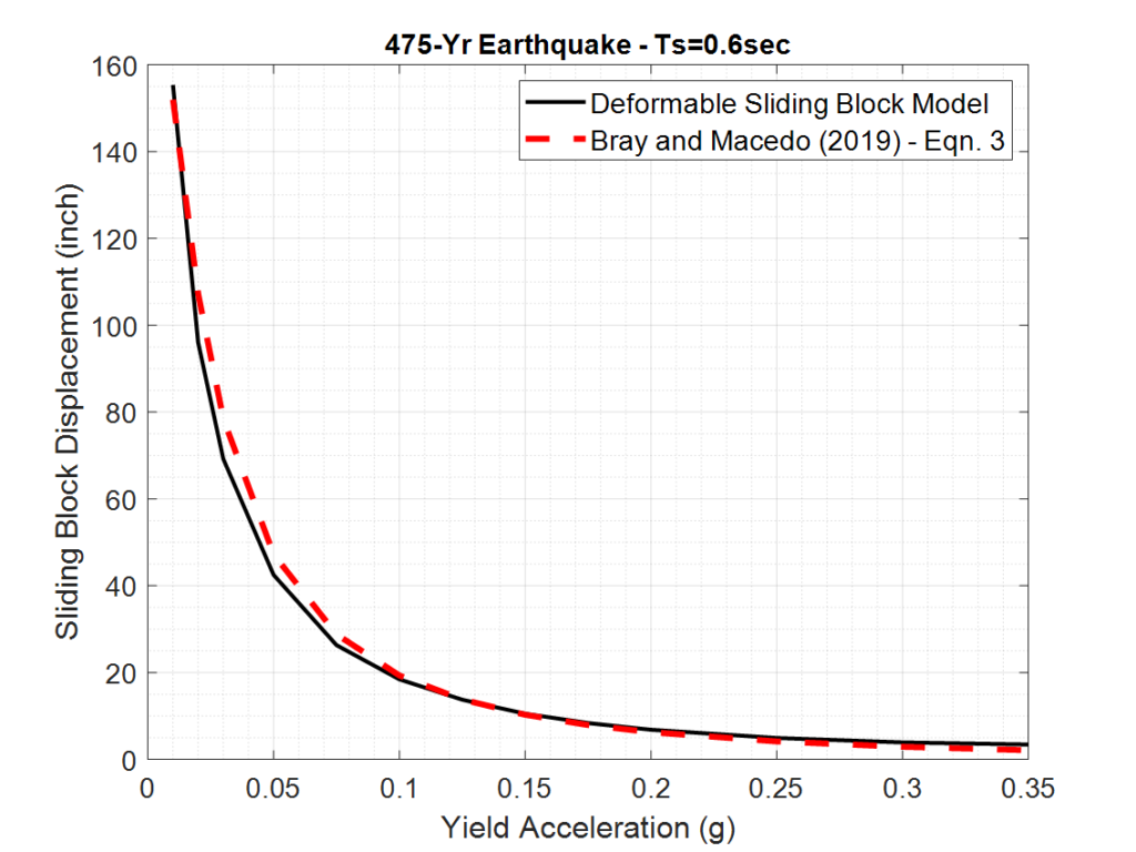
In addition, the results of the MATLAB code was compared against the approach proposed by Bray and Macedo (2019). A suite of 7 ground motions spectrally-matched to a site-specific target acceleration response spectrum was selected. Yield accelerations in the range 0f 0.01g to 0.35g were considered. The analyses considered a soil mass with natural period of 0.6 second. The computed slope displacement-yield acceleration graph is compared against those estimated by Eqn. 3 presented in Bray and Macedo (2019) for “Ordinary Ground Motions”. The input parameters for the Bray and Macedo (2019) approach, i.e., k_y, T_s, Sa(1.3Ts), M_w were similar to those used in the MATLAB code. Figure 6 compares the analysis outputs. The results indicated that there is a good agreement between the MATLAB code results and those predicted by Bray and Macedo (2019).
Supplemental MATLAB File
As noted earlier, in the MATLAB file above sliding is calculated in one direction (downslope) only, and sliding in the opposite direction (upslope) is neglected. This is valid for estimation of lateral seismic movement of slopes where the soil block downslope movement is permanent and sliding in the opposite direction is not possible due to the significant resistance from the upslope soil media. If one is interested to find out how the sliding time history would be if sliding could occur in both directions, the MATLAB code below can be used:
Download link:
Two-way Sliding Matlab Code
It is to be noted that this MATLAB file should not be used for estimation of slope movements because of the reasons discussed above. The file is uploaded here for the use of those who are interested to further investigate how the response of the sliding mass would be if sliding could occur in both + and – directions.