This article intends to shed light on application of Rayleigh and numerical damping in finite element and finite difference analyses.

As you all know, there are two types of damping in a system subjected to dynamic loads; (1) material damping, and (2) radiation damping. Material damping is the dissipated energy due to the yielding of soil material and significant hysteretic behavior. Radiation damping is the dissipated energy due to the propagation of motion into the semi-infinite half space. It is important to note that neither Rayleigh damping nor numerical damping are classified as material/radiation type damping. These two dampings do NOT physically exist in a system subjected to dynamic loads, but interestingly they are required to successfully complete a numerical analysis. The following sections provide an overview of each type of damping and explain why these unreal dampings should be used in advanced numerical simulations.

Rayleigh Damping

Based on Newton’s Law, for any object subjected to seismic loading the equilibrium equation in the form of matrix is;

{\bf M}\ddot{\textit{\textbf Y}}+{\bf C}\dot{\textit {\textbf Y}}+{\bf K}{\textit {\textbf Y}}=-{\bf M}\ddot{\textit{\textbf Y}}_g

where \bf M, \bf C , and \bf K are the system mass, damping and stiffness matrices, respectively, \ddot{\textit{\textbf Y}}_g is the input ground motion acceleration applied at the base of system, and \textit {\textbf Y} is the relative displacement vector with respect to the base of the system.

Note that the damping matrix for an earth system is zero (\bf C = 0) because there is no dashpot or any kind of physical damping component within a soil deposit. Therefore the equilibrium equation for a geotechnical system is given as,

{\bf M}\ddot{\textit{\textbf Y}}+{\bf K}{\textit {\textbf Y}}=-{\bf M}\ddot{\textit{\textbf Y}}_g

In the equation above, material damping is simulated by the constitutive model which simulates soil hysteretic stress-strain response, and Radiation damping is simulated by devloping the finite element/difference of the semi-infinite half space. Now the question is why Rayleigh Damping is deemed necessary while both material and radiation damping are already accounted for in the analysis.

The reason for using Rayleigh Damping in simulation of a geotechnical system is twofold:

1. To account for energy dissipation at very small shear strain levels (typically \gamma \leq 10^{-6} ): Note that even at low deformation levels, soil behavior is irreversible. Constitutive models may not be capable of appropriately simulating this when stress-state is located within the yield surface. In the literature, it is recommended to apply Rayleigh damping and introduce a damping ratio ({\zeta}) in the range of 0.5 to 2.0% to account for energy dissipation at low shear strains. Typical damping-shear strain curves such as those proposed by Seed et al. (1986) and Vucetic and Dobry (1991) can be used to determine appropriate damping ratio. Based on these curves, damping ratio ({\zeta}) of roughly 0.5% for sands and 1.0% for clays seem to be adequate.
2. To damp out the spurious oscillations occurring in high frequency domain: Note that both finite element and finite difference methods provide numerical solution not analytical solution for the equilibrium equation in which the external force is earthquake motion with discrete data points. According to the literature, without introducing any artificial damping such as Rayleigh damping, some high frequency noises develop in the model which often cause serious problem in the numerical analysis by triggering instability of the computation process, especially when the system has large degree of freedoms. This will be further elaborated in the next section.

Rayleigh damping is introduced to the equilibrium equation by the component {\bf C}\dot{\textit {\textbf Y}} where the damping matrix {\bf C} is given by a portion of the mass matrix {\bf M} and a portion of the stiffness matrix {\bf K}. The equation below presents the Rayleigh damping formulation;

{\bf C}=\alpha {\bf M} + \beta {\bf K}

where \alpha and \beta, respectively, represent the mass and stiffness proportional damping coefficients. Rayleigh damping of vibration mode i ( \zeta_i ) is given by:

\zeta_i = \frac{1}{2} (\frac{\alpha}{\omega_i}+\beta \omega_i)

where \omega_i is the undamped natural frequency of i^{th} mode shape.  To incorporate the above equation into the equilibrium equation, a modal response analysis in frequency domain is required to compute \zeta_i and \omega_i. However, this is NOT feasible because both finite element and finite difference methods are implemented in time domain. To  overcome this issue, several researcher proposed to conceptually enforce a Rayleigh damping curve that matches a prescribed modal damping (\zeta) at two special frequency points. These two frequencies will be discussed shortly herein. Using this criterion by solving the above equation for a given damping ratio and two frequencies, \alpha and \beta can be calculated by the following equations;

{\alpha=2 \zeta \frac{ \omega_i \omega_j}{\omega_i+ \omega_j}}

{\beta=2 \zeta \frac{ 1}{\omega_i+ \omega_j}}

where \zeta is damping ratio (typically 0.5 to 2.0 %) representing material damping at very low shear strains, i.e.,  \gamma \leq 10^{-6}.  \omega_i and \omega_j are the fundamental frequencies of i^{th} and j^{th} vibration modes, respectively. The choice of these two frequencies has been widely studied by several researchers. Hudson et al. (1994) proposed to set the first frequency equal to the natural frequency of soil layer (\omega_i = 2 \pi V_s/4H ) and the second frequency equal to n\omega_i where n is the closest odd number greater than the ratio of the fundamental frequency of the input motion at the model base and natural frequency of soil layer. For example, if natural frequencies of input motion and soil layer are 3.3 and 1.0 Hz, respectively, the ratio would be 3.3/1.0=3.3; hence, n =5.0.  Note that n is desired to be odd number because i^{th} natural frequency of a soil layer is odd multiples of frequency of the fundamental vibration mode of the soil layer. Equation below presents the i^{th} natural frequency of a soil layer with height H and average shear wave velocity V_s :

f_i=\frac{V_s}{4H} (2i+1)

Numerical Damping

In order to solve the equilibrium equation by numerical methods, it is necessary to introduce equations relating \ddot{\it{\bf Y}}, \dot{\it{\bf Y}}, and \it{\bf Y}. The Newmark family of implicit time integration schemes is generally implemented in goetechnical computer programs to provide the required equations.  Note that these equations are originally formulated based on Taylor series expansions for displacement, velocity, and acceleration by truncating the fourth time-derivative and higher from the expansions.

The Newmark-\beta time integration algorithms require the displacement and velocity to be updated as follows at time step t+\Delta t;

Y^{t+\Delta t}=Y^{t}+\dot{Y}^t\Delta t+[(\frac{1}{2}-\beta)\ddot{Y}^{t}+\beta\ddot{Y}^{t+\Delta t}] {\Delta t}^2

\dot{Y}^{t+\Delta t}=\dot{Y}^{t}+[(1-\gamma)\ddot{Y}^{t}+\gamma\ddot{Y}^{t+\Delta t}] {\Delta t}

The variables \beta and \gamma are numerical parameters that control both the stability of the method and the amount of numerical damping introduced into the system by the method. In order to obtain a stable solution from the above equations, the following conditions must apply:

\gamma \geq 0.5 ,     \beta \geq \frac{1}{4}(\frac{1}{2}+\gamma)^2

If \gamma = 0.5 and \beta = 0.25 are used, there will be no numerical damping at any frequency; however, for \gamma  greater than 0.5 numerical damping is introduced. Note that the larger \gamma is, the greater the numerical damping becomes.

It is surely desirable to avoid introducing numerical damping in a simulation; however, it is well-established that using \gamma = 0.5 and \beta = 0.25, i.e., no numerical damping, results in generation of high frequency noises that often cause serious problems in computations by triggering instability of the computation process, especially when the system has large degree-of-freedom and/or nonlinear material behavior is considered (Honda and Sawada, 2000).  To remove these spurious oscillations, it is generally recommended to; (i) introduce Rayleigh Damping, and/or (ii) use Newmark parameters of \gamma = 0.6 and \beta = 0.3025. These parameters have been shown to adequately damp out noises and stabilize the integration scheme without introducing considerable amount of damping to the system.

A hypothetical example is provided herein to illustrate the effectiveness of application of Rayleigh  damping and numerical damping in a seismic finite element analysis. In this example, performance of a 20-foot deep soil layer subjected to an earthquake loading is assessed for each of the following scenarios:

• Scenario #1: no Rayleigh damping and no numerical damping, i.e., Newmark parameters of \gamma = 0.5 and \beta = 0.25;
• Scenario #2: Rayleigh damping with 1% damping ratio and no numerical damping;
• Scenario #3: no Rayleigh damping but with numerical damping, i.e., Newmark parameters of \gamma = 0.6 and \beta = 0.3025;
• Scenario #4: Rayleigh damping with 1% damping ratio and with numerical damping, i.e., Newmark parameters of \gamma = 0.6 and \beta = 0.3025;

All numerical analyses are performed using the finite element computer program, PLAXIS 2D. Figure 1 shows the FE model and the input soil parameters.

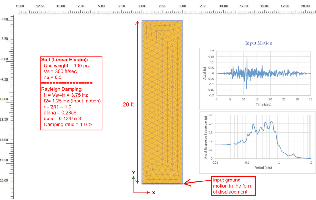
Figure 2 presents the computed acceleration time histories at the ground surface and the base of model, i.e., depth =20 feet, for all four scenarios. For clarity, time history of input ground motion is also shown in the figure. Per the results of scenario #1, a considerable amount of spurious noises develop when no Rayleigh damping or numerical damping is introduced to the analysis. In scenario #2, Rayleigh damping successfully damps out the noises at the ground surface; however, considerable noises still develop at the base. It appears that Rayleigh damping does not remove the noises at locations close to the model base. This might be considered sufficient since model base is generally set to be deep enough to minimize base boundary conditions effect, and additionally the seismic responses at shallow depths are generally of interest in a numerical simulation. However, for a large scale numerical model with highly nonlinear material these noises at the base may cause numerical instability that results in convergence failure. Scenario #3 shows how effectively introducing a small amount of numerical damping (\gamma = 0.6 and \beta = 0.3025) removes the spurious oscillations over the entire soil layer. By comparing the computed base motion against the actual input motions, it is noted that the numerical damping does not alter the frequency content and the amplitude of the input ground motion. Scenario #4 shows that introducing both Rayleigh damping and numerical damping also adequately damps out noises. However, note that although the frequency content of the motions remains unchanged, by comparing the ground surface motion against that in scenario #2 and 3 the amplitudes of the motion decrease noticeably. This implies that Rayleigh damping and numerical damping should NOT be both introduced to an analysis, unless Rayleigh damping is intended to simulate additional material damping at low shear strains.

Concluding Remarks

The following notes should be considered when Rayleigh or numerical damping is introduced to a finite element/difference analysis of a geotechnical system:

1. As discussed earlier in this article, the external load in the equilibrium equation is an earthquake motion with discrete data points. By application of numerical methods to solve the equilibrium equation, some spurious oscillations inevitably develop in the system response. In order to remove these noises, it is essential to introduce either Rayleigh damping or numerical damping.
2. Rayleigh damping is used to:
   111(i) damp out the spurious noises;
   111(ii) simulate material damping at low shear strains when soil is in elastic state.
   Numerical damping is merely used to damp out the noises. It is not intended to simulate any other type of system damping.
3. Rayleigh damping is shown to be incapable of removing noises at locations close to the model base. These noises may cause analysis convergence failure for large-scale highly nonlinear models. Numerical damping (\gamma = 0.6 and \beta = 0.3025) better removes noises within the entire system.
4. Rayleigh damping and numerical damping must NOT be both applied to a model unless Rayleigh damping is intended to simulate material damping at low shear strains.
5. Rayleigh damping introduces the component, {\bf C}\dot{\textit {\textbf Y}}, into the equilibrium equation. Note that this component is representing a hypothetical force that does not physically exist in a geotechnical system. Therefore, in my opinion if it is judged that material damping at low shear strains is negligible for a system, it is much preferred to apply numerical damping rather than Rayleigh damping.